Ethan's BGGN 213 Portfolio
Class work for bioinformatics
Class 08: Breast Cancer Analysis Project
Ethan Ashley (PID: A15939817) 2025-10-24
- Background
- Data Import
- Exploratory Data Analysis
- Principal Component Analysis
- Hierarchical Clustering
- Combining Methods
- Prediction
Background
The goal of this mini-project is for you to explore a complete analysis using the unsupervised learning techniques covered in class. We will extend what we’ve learned by combining PCA as a preprocessing step to clustering using data that consist of measurements of cell nuclei of human breast masses. This expands on our RNA-Seq analysis from last day.
The data itself comes from the Wisconsin Breast Cancer Diagnostic Data Set first reported by K. P. Benne and O. L. Mangasarian: “Robust Linear Programming Discrimination of Two Linearly Inseparable Sets”.
Values in this data set describe characteristics of the cell nuclei present in digitized images of a fine needle aspiration (FNA) of a breast mass.
Data Import
Importing the Wisconsin Cancer data set. Make sure not to include the patient IDs or the pathologists diagnoses in the data that we analyze below.
fna.data <- "WisconsinCancer.csv"

wisc.df <- read.csv(fna.data, row.names = 1)

# We can use -1 here to remove the first column containing the pathologist classifications
diagnosis <- wisc.df$diagnosis
wisc.data <- wisc.df[,-1]
wisc.data <- wisc.data[,-31]
Exploratory Data Analysis
Q1. How many observations are in this dataset?
There are 569 observations in the dataset.
nrow(wisc.data)
## [1] 569
Q2. How many of the observations have a malignant diagnosis?
There are 212 twelve observations with a malignant diagnosis.
sum(diagnosis == "M")
## [1] 212
table(wisc.df$diagnosis) #alternative method shown in class
##
##   B   M
## 357 212
**Q3. How many variables/features in the data are suffixed with _mean?**
There are 10 variables in the data that are suffixed with _mean.
length(grep("_mean", colnames(wisc.data)))
## [1] 10
Principal Component Analysis
The main function in base R for PCA is prcomp(). It has optional
inputs scale and center.
In general we want to scale and center our data prior to PCA to ensure that each feature contributes equally to the analysis, preventing variables with larger scales from dominating the principal components.
# Check column means and standard deviations
colMeans(wisc.data)
##             radius_mean            texture_mean          perimeter_mean
##            1.412729e+01            1.928965e+01            9.196903e+01
##               area_mean         smoothness_mean        compactness_mean
##            6.548891e+02            9.636028e-02            1.043410e-01
##          concavity_mean     concave.points_mean           symmetry_mean
##            8.879932e-02            4.891915e-02            1.811619e-01
##  fractal_dimension_mean               radius_se              texture_se
##            6.279761e-02            4.051721e-01            1.216853e+00
##            perimeter_se                 area_se           smoothness_se
##            2.866059e+00            4.033708e+01            7.040979e-03
##          compactness_se            concavity_se       concave.points_se
##            2.547814e-02            3.189372e-02            1.179614e-02
##             symmetry_se    fractal_dimension_se            radius_worst
##            2.054230e-02            3.794904e-03            1.626919e+01
##           texture_worst         perimeter_worst              area_worst
##            2.567722e+01            1.072612e+02            8.805831e+02
##        smoothness_worst       compactness_worst         concavity_worst
##            1.323686e-01            2.542650e-01            2.721885e-01
##    concave.points_worst          symmetry_worst fractal_dimension_worst
##            1.146062e-01            2.900756e-01            8.394582e-02
apply(wisc.data,2,sd)
##             radius_mean            texture_mean          perimeter_mean
##            3.524049e+00            4.301036e+00            2.429898e+01
##               area_mean         smoothness_mean        compactness_mean
##            3.519141e+02            1.406413e-02            5.281276e-02
##          concavity_mean     concave.points_mean           symmetry_mean
##            7.971981e-02            3.880284e-02            2.741428e-02
##  fractal_dimension_mean               radius_se              texture_se
##            7.060363e-03            2.773127e-01            5.516484e-01
##            perimeter_se                 area_se           smoothness_se
##            2.021855e+00            4.549101e+01            3.002518e-03
##          compactness_se            concavity_se       concave.points_se
##            1.790818e-02            3.018606e-02            6.170285e-03
##             symmetry_se    fractal_dimension_se            radius_worst
##            8.266372e-03            2.646071e-03            4.833242e+00
##           texture_worst         perimeter_worst              area_worst
##            6.146258e+00            3.360254e+01            5.693570e+02
##        smoothness_worst       compactness_worst         concavity_worst
##            2.283243e-02            1.573365e-01            2.086243e-01
##    concave.points_worst          symmetry_worst fractal_dimension_worst
##            6.573234e-02            6.186747e-02            1.806127e-02
Scaling and centering is advisable with this dataset.
# Perform PCA on wisc.data by completing the following code
wisc.pr <- prcomp(wisc.data, scale. = TRUE)
Q4. From your results, what proportion of the original variance is captured by the first principal components (PC1)?
44.27% of the original variance is accounted for by PC1.
Q5. How many principal components (PCs) are required to describe at least 70% of the original variance in the data?
3 PCs are required to describe at least 70% of the original variance in the dataset.
Q6. How many principal components (PCs) are required to describe at least 90% of the original variance in the data?
7 PCs are required to describe at least 90% of the original variance in the dataset.
summary(wisc.pr)
## Importance of components:
##                           PC1    PC2     PC3     PC4     PC5     PC6     PC7
## Standard deviation     3.6444 2.3857 1.67867 1.40735 1.28403 1.09880 0.82172
## Proportion of Variance 0.4427 0.1897 0.09393 0.06602 0.05496 0.04025 0.02251
## Cumulative Proportion  0.4427 0.6324 0.72636 0.79239 0.84734 0.88759 0.91010
##                            PC8    PC9    PC10   PC11    PC12    PC13    PC14
## Standard deviation     0.69037 0.6457 0.59219 0.5421 0.51104 0.49128 0.39624
## Proportion of Variance 0.01589 0.0139 0.01169 0.0098 0.00871 0.00805 0.00523
## Cumulative Proportion  0.92598 0.9399 0.95157 0.9614 0.97007 0.97812 0.98335
##                           PC15    PC16    PC17    PC18    PC19    PC20   PC21
## Standard deviation     0.30681 0.28260 0.24372 0.22939 0.22244 0.17652 0.1731
## Proportion of Variance 0.00314 0.00266 0.00198 0.00175 0.00165 0.00104 0.0010
## Cumulative Proportion  0.98649 0.98915 0.99113 0.99288 0.99453 0.99557 0.9966
##                           PC22    PC23   PC24    PC25    PC26    PC27    PC28
## Standard deviation     0.16565 0.15602 0.1344 0.12442 0.09043 0.08307 0.03987
## Proportion of Variance 0.00091 0.00081 0.0006 0.00052 0.00027 0.00023 0.00005
## Cumulative Proportion  0.99749 0.99830 0.9989 0.99942 0.99969 0.99992 0.99997
##                           PC29    PC30
## Standard deviation     0.02736 0.01153
## Proportion of Variance 0.00002 0.00000
## Cumulative Proportion  1.00000 1.00000
Interpreting PCA results
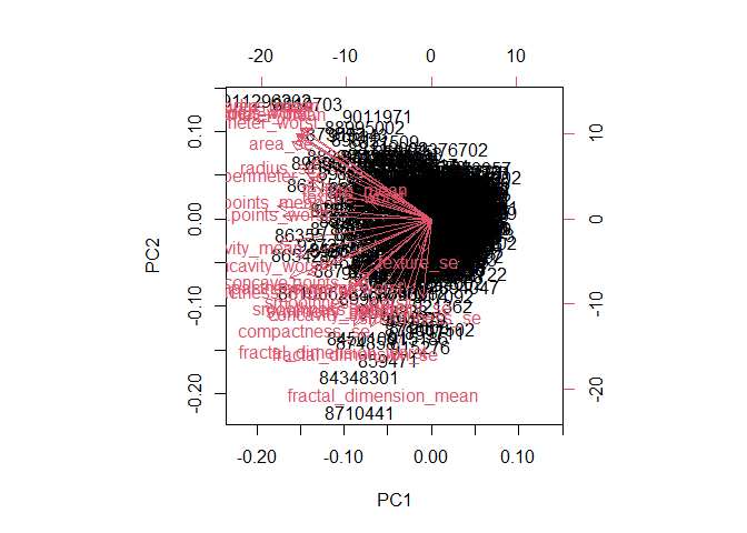
Q7. What stands out to you about this plot? Is it easy or difficult to understand? Why?
This plot is very messy and difficult to read. It is not possible to tell which points come from which diagnosis group.
biplot(wisc.pr)
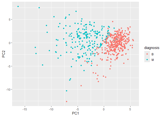
Let’s make our main results figure - the “PC plot” or “score plot”.
library(ggplot2)

ggplot(wisc.pr$x) + aes(PC1, PC2, color = diagnosis) + geom_point()
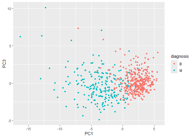
Q8. Generate a similar plot for principal components 1 and 3. What do you notice about these plots?
There is still good clustering of the benign and malignant tumors. Since PC3 explains less of the variance than PC2, it doesn’t do quite as good of a job of separating the two groups.
ggplot(wisc.pr$x) + aes(PC1, PC3, color = diagnosis) + geom_point()
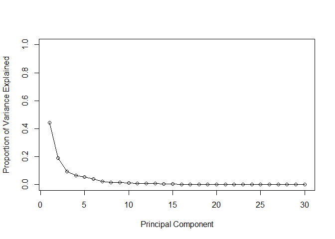
Variance Explained
# Calculate variance of each component
pr.var <- wisc.pr$sdev^2
head(pr.var)
## [1] 13.281608 5.691355 2.817949 1.980640 1.648731 1.207357
# Variance explained by each principal component: pve
pve <- pr.var / sum(pr.var)

# Plot variance explained for each principal component
plot(pve, xlab = "Principal Component",
     ylab = "Proportion of Variance Explained",
     ylim = c(0, 1), type = "o")
Q9. For the first principal component, what is the component of the loading vector (i.e. wisc.pr$rotation[,1]) for the feature concave.points_mean? This tells us how much this original feature contributes to the first PC.
The component of the loading vector for PC1 for the feature concave.points_mean is -0.26085376.
wisc.pr$rotation[,1]
##             radius_mean            texture_mean          perimeter_mean
##             -0.21890244             -0.10372458             -0.22753729
##               area_mean         smoothness_mean        compactness_mean
##             -0.22099499             -0.14258969             -0.23928535
##          concavity_mean     concave.points_mean           symmetry_mean
##             -0.25840048             -0.26085376             -0.13816696
##  fractal_dimension_mean               radius_se              texture_se
##             -0.06436335             -0.20597878             -0.01742803
##            perimeter_se                 area_se           smoothness_se
##             -0.21132592             -0.20286964             -0.01453145
##          compactness_se            concavity_se       concave.points_se
##             -0.17039345             -0.15358979             -0.18341740
##             symmetry_se    fractal_dimension_se            radius_worst
##             -0.04249842             -0.10256832             -0.22799663
##           texture_worst         perimeter_worst              area_worst
##             -0.10446933             -0.23663968             -0.22487053
##        smoothness_worst       compactness_worst         concavity_worst
##             -0.12795256             -0.21009588             -0.22876753
##    concave.points_worst          symmetry_worst fractal_dimension_worst
##             -0.25088597             -0.12290456             -0.13178394
Hierarchical Clustering
# Scale the wisc.data data using the "scale()" function
data.scaled <- scale(wisc.data)
data.dist <- dist(data.scaled)
wisc.hclust <- hclust(data.dist, method="complete")
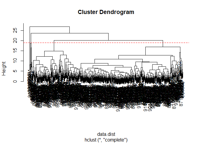
Q10. Using the plot() and abline() functions, what is the height at which the clustering model has 4 clusters?
A height of 19 appears to lead to 4 clusters.
plot(wisc.hclust)
abline(h=19, col="red", lty=2)
Using Different Methods
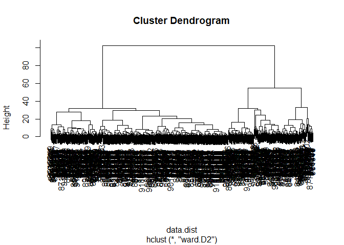
Q12. Which method gives your favorite results for the same data.dist dataset? Explain your reasoning.
The method ward.D2 produces my favorite results for the data.dist. It is the easiest of the various options to tell where branches of clusters form.
wisc.hclust <- hclust(data.dist, method="ward.D2")

plot(wisc.hclust)
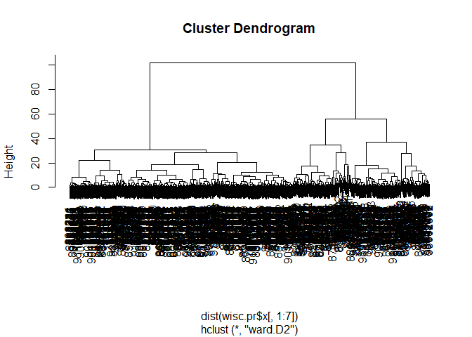
Combining Methods
wisc.pr.hclust <- hclust(dist(wisc.pr$x[,1:7]), method="ward.D2")

plot(wisc.pr.hclust)
grps <- cutree(wisc.pr.hclust, h=70)
table(grps)
## grps
##   1   2
## 216 353
table(grps, diagnosis)
##     diagnosis
## grps   B   M
##    1  28 188
##    2 329  24
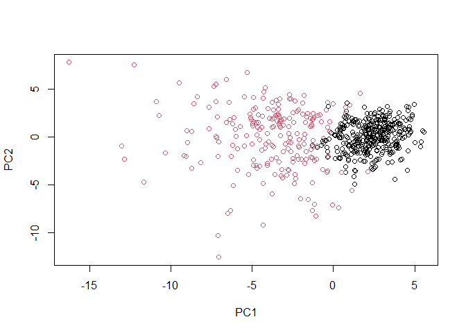
plot(wisc.pr$x[,1:2], col=grps)
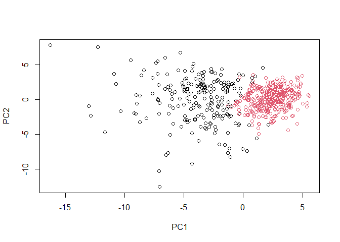 There are 188
true positives and 28 false positives in the malignant group. There are
329 true positives and 24 false positives in the benign group.
There are 188
true positives and 28 false positives in the malignant group. There are
329 true positives and 24 false positives in the benign group.
g <- as.factor(grps)
levels(g)
## [1] "1" "2"
g <- relevel(g,2)
levels(g)
## [1] "2" "1"
# Plot using our re-ordered factor
plot(wisc.pr$x[,1:2], col=g)
library(rgl)
plot3d(wisc.pr$x[,1:3], xlab="PC 1", ylab="PC 2", zlab="PC 3", cex=1.5, size=1, type="s", col=grps)
Q13. How well does the newly created model with four clusters separate out the two diagnoses?
In general, the newly created model is fairly accurate. However, in a clinical setting, the false negatives and positives would not be desirable.
## Use the distance along the first 7 PCs for clustering i.e. wisc.pr$x[, 1:7]
wisc.pr.hclust <- hclust(dist(wisc.pr$x[, 1:7]), method="ward.D2")

wisc.pr.hclust.clusters <- cutree(wisc.pr.hclust, k=2)

table(wisc.pr.hclust.clusters, diagnosis)
##                        diagnosis
## wisc.pr.hclust.clusters   B   M
##                       1  28 188
##                       2 329  24
Q14. How well do the hierarchical clustering models you created in previous sections (i.e. before PCA) do in terms of separating the diagnoses? Again, use the table() function to compare the output of each model (wisc.km$cluster and wisc.hclust.clusters) with the vector containing the actual diagnoses.
These other methods appear to do a fairly good job of classifying the data.
wisc.km <- kmeans(wisc.data, 2)

table(wisc.km$cluster, diagnosis)
##    diagnosis
##       B   M
##   1 356  82
##   2   1 130
wisc.hclust.clusters <- cutree(wisc.hclust, k=2)

table(wisc.hclust.clusters, diagnosis)
##                     diagnosis
## wisc.hclust.clusters   B   M
##                    1  20 164
##                    2 337  48
Prediction
#url <- "new_samples.csv"
url <- "https://tinyurl.com/new-samples-CSV"
new <- read.csv(url)
npc <- predict(wisc.pr, newdata=new)

plot(wisc.pr$x[,1:2], col=g)
points(npc[,1], npc[,2], col="blue", pch=16, cex=3)
text(npc[,1], npc[,2], c(1,2), col="white")
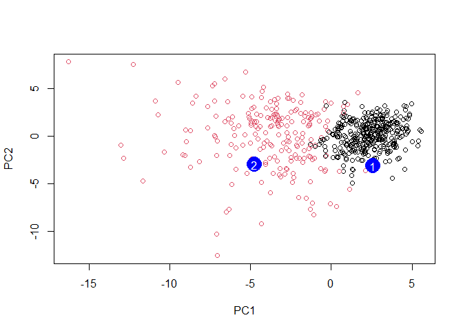
Q16. Which of these new patients should we prioritize for follow up based on your results?
I think we should prioritize patient 2 as they fall into the malignant tumor group.